ベイズの定理とモンティ・ホール問題

昨今、一部界隈では「ベイズの定理」を知っているか否かで、データサイエンティストがホンモノかを見極めているらしい。
ここでは公式の確認と問題例とともに「ベイズの定理」を復習しようと思う。

まずベイズの定理とは、
事象A, 事象Bが発生する確率をそれぞれP(A), P(B)とし、
P(A|B)：Bが真であるとき、Aが発生する確率
P(B|A)：Aが真であるとき、Bが発生する確率
とした場合、となる公式である。

また、モンティ・ホール問題とは

①、②、③の箱のうち、どれか1つだけに豪華賞品がある。あなたはドア①を選択し、司会者がドア②が開けたとする。
このとき、あなたはドア①のままを選ぶか、ドア③に変更するか？

という問題である。ここで求めたい確率は、

• ドア②が開いた後に、ドア①に豪華賞品がある確率
• ドア②が開いた後に、ドア③に豪華賞品がある確率

○解説
[1]ドア①に豪華賞品がある場合
P(A) ： ドア②が開く確率 = ドア①が当たり(1/6) +ドア②が当たり(0) +ドア③が当たり(1/3) = 1/2
P(B) ： ドア①に豪華賞品がある確率 （事前確率）= 1/3
P(A|B) ： ドア①に豪華賞品があった場合に、ドア②を開く確率（条件確率）=1/2
P(B|A) ： ドア②が開いた後に、ドア①に豪華賞品がある確率 = P(A|B)*P(B)/P(A) = 1/3 ★ベイズの定理

[2]ドア③に豪華賞品がある場合
P(A) ： ドア②が開く確率 = 1/2
P(B) ： ドア③に豪華賞品がある確率 （事前確率）= 1/3
P(A|B) ： ドア③に豪華賞品があった場合に、ドア②を開く確率（条件確率）=1/1
P(B|A) ： ドア②が開いた後に、ドア③に豪華賞品がある確率 = P(A|B)*P(B)/P(A) = 2/3 ★ベイズの定理

[1], [2]より

• ドア① に豪華賞品がある確率は、1/3
• ドア③ に豪華賞品がある確率は、2/3

よって、モンティ・ホール問題では、最初に選んだ選択肢を変更する方が、豪華賞品が当たる確率が上がる。

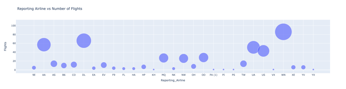
plotlyによる可視化

バブルチャートによる可視化

import plotly.express as px
fig = px.scatter(bub_data, x="Reporting_Airline", y="Flights", size="Flights",
                 hover_name="Reporting_Airline", title='Reporting Airline vs Number of Flights', size_max=60)
fig.show()

バブルチャート

pythonクラスの備忘録

pythonクラスにおいて、クラス変数とインスタンス変数の違いについて説明する。
まず、以下のようなクラスを定義する。

class ClassVal:
    x = "ClassVal"

class InstanceVal:
    def __init__(self):
        self.x = "InstanceVal"

cls_Val = ClassVal()
ins_Val = InstanceVal()

この時、インスタンス化されたcls_Valのクラス変数、ins_Valのインスタンス変数はいずれも表示できる

print(cls_Val.x) # ClassVal
print(ins_Val.x) # InstanceVal

一方、ClassValのクラス変数は表示できるが、InstanceValのインスタンス変数は表示出来ない

print(ClassVal.x) # class変数に設定されているので、表示できる
print(InstanceVal.x) # instance化しないと表示できないため、エラーとなる

Regrssion Plots

今回の記事では、散布図とその近似曲線及び領域を描画する。
まず、下記のようなdfを作成する。

df_tot

seabornのregplotを用いると、簡単に回帰直線を描ける。

import seaborn as sns
plt.figure(figsize=(15, 10))
sns.set(font_scale=1.5)
ax = sns.regplot(x='year', y='total', data=df_tot, color='green', marker='+', scatter_kws={'s': 200})
ax.set(xlabel='Year', ylabel='Total Immigration')
ax.set_title('Total Immigration to Canada from 1980 - 2013')

regplot2

regplotの引数は下記の通り。

seaborn.regplot(x, y, data=None, x_estimator=None, x_bins=None, x_ci='ci',
　　　　　　　　　 scatter=True, fit_reg=True, ci=95, n_boot=1000, units=None, 
                order=1, logistic=False, lowess=False, robust=False, logx=False,
                x_partial=None, y_partial=None, truncate=False, dropna=True,
                x_jitter=None, y_jitter=None, label=None, color=None, marker='o', 
                scatter_kws=None, line_kws=None, ax=None)

主要な引数

• ci：回帰を行う際の信頼区間 (%) を指定 (デフォルトは95%)
• order：1 以上の数値を指定すると、numpy.polyfit を用いて多項式回帰を行う (デフォルトは1)

参考：Seaborn で散布図・回帰モデルを可視化する

箱ひげ図の基本

箱ひげ図はデータの分布を簡単に確認でき、分布同士を比較する場合に非常に便利である。

○箱ひげ図で確認するポイント

• 箱ひげ図の全長から分かるばらつき
• 中央値と平均値のズレ
• 外れ値からの外れ具合

○外れ値が発生する確率

データが正規分布に従うと仮定した場合、

• 中央値=平均値
• 第一四分値の確率(第三四分値の確率)=Zσ=0.67σ

外れ値にならない範囲は、25%点(75%点)±1.5×IQR ＝ 0.67σ + 1.5*1.34 σ= ±2.67σ →確率としては99.2% (±3σは99.7%)
つまり、箱ひげ図で外れ値となる確率は0.8% (12500分の1)

3σ

参考：箱ひげ図(ボックスプロット)の外れ値 どのくらいの確率で外れる？

「棒グラフ」と「円グラフ」の使い分け

入社してすぐの研修で、データサイエンティストの3大ご法度として「円グラフの利用」が上げられていた。
今回は、なぜ円グラフが問題視されるかを深掘っていく。

○円グラフの課題
割合の変化が微小である時、その変化を捉えにくい。

円グラフ

棒グラフ

上の円グラフと下の棒グラフは対応するが、円グラフではその割合の変化は捉えずらい。
一方で、棒グラフでは容易にその推移が確認できる。
よって、データの割合が極端に変動しない限りは、円グラフは使わないほうがよい。

参考：Survey Results: Reporting via Pie Charts or Bar Graphs

matplotlibの基礎知識

matplotlibは次の3層で構成される

1.Scripting Layer

• pyplot
• df.plot()

2.Artist Layer

• ax = df.plot()
• グラフに表示されるものは全てArtist

  

  Artist

3.Backend Layer

• backend_bases

matplotlibの階層構造を簡潔に表した図。

階層構造

この図から読み取れること

• FigureオブジェクトにAxesオブジェクトが属している
• AxesオブジェクトにはAxisオブジェクトが属している

参考

• 早く知っておきたかったmatplotlibの基礎知識、あるいは見た目の調整が捗るArtistの話

○棒グラフの例1. 重なりを透過した棒グラフ

# create a dataframe of the countries of interest (cof)
df_cof = df_can.loc[['Greece', 'Albania', 'Bulgaria'], years]

# transpose the dataframe
df_cof = df_cof.transpose() 

# let's get the x-tick values
count, bin_edges = np.histogram(df_cof, 15)

# Un-stacked Histogram
df_cof.plot(kind ='hist',
            figsize=(10, 6),
            bins=15,
            alpha=0.35,
            xticks=bin_edges,
            color=['coral', 'darkslateblue', 'mediumseagreen']
            )

plt.title('Histogram of Immigration from Greece, Albania, and Bulgaria from 1980 - 2013')
plt.ylabel('Number of Years')
plt.xlabel('Number of Immigrants')

plt.show()

出力

hist

○棒グラフの例2. 棒グラフへ数値埋め込み

### type your answer here
df_top15.plot(kind='barh',figsize=(12,12),color = 'steelblue')
plt.xlabel('Number of Immigrants')
plt.title('Top 15 Conuntries Contributing to the Immigration to Canada between 1980 - 2013')

# annotate value labels to each country
for index, value in enumerate(df_top15): 
    label = format(int(value), ',') # format int with commas

# place text at the end of bar (subtracting 47000 from x, and 0.1 from y to make it fit within the bar)
    plt.annotate(label, xy=(value - 47000, index - 0.10), color='white')

plt.show()

出力

bar with numbers

○Subplotsの基本形
典型的な記述方法は以下の通り。

fig = plt.figure() # create figure
ax = fig.add_subplot(nrows, ncols, plot_number) # create subplots

subplots

○散布図と近似直線の可視化

x = df_tot['year']      # year on x-axis
y = df_tot['total']     # total on y-axis
fit = np.polyfit(x, y, deg=1)

df_tot.plot(kind='scatter', x='year', y='total', figsize=(10, 6), color='darkblue')

plt.title('Total Immigration to Canada from 1980 - 2013')
plt.xlabel('Year')
plt.ylabel('Number of Immigrants')

# plot line of best fit
plt.plot(x, fit[0] * x + fit[1], color='red') # recall that x is the Years
plt.annotate('y={0:.0f} x + {1:.0f}'.format(fit[0], fit[1]), xy=(2000, 150000))

plt.show()

# print out the line of best fit
'No. Immigrants = {0:.0f} * Year + {1:.0f}'.format(fit[0], fit[1]) 

plot line